Supermongo help

Supermongo (SM) is an interactive plotting programme with a flexible command language. It's reasonably easy to use and fairly powerful. This page is intended to help people start using SM without having to read through the manual or online help too much.

Starting SM

	> xhost +xray02

	> setenv DISPLAY [your hostname]:0.0

	Hello Duncan, please give me a command

Basic commands

help
help command

Access the online help. The first command will provide a list of relevant topics, while the second will provide help on a specific topic.

data "file.dat"

Open the named file for reading. This must be done before a read command can be issued. Data files must be numbers only (no header lines) with columns separated by spaces, tabs or commas.

read { x 1 y 2 z 3 }

Read three columns from the open data file. For each column which is to be read in you must provide a vector name (x, y, z etc.) and a column number. It is possible to read less than the total number of columns in a file using this command.

limits x y
limits x 4 5
limits 100 200 y
limits 100 200 4 5


Set the plot limits in the current window. The first command sets the x-range to the range of vector x, and the y-range to the range of vector y. You can replace any vector in this command with a specific range.

box
box 1 3
box 1 1 0 0

Draw a box around the plot area in the current window. The first command draws a box with ticks and labels on the bottom and left hand side, and ticks only on the top and right hand sides (this is the default). The command can also be used to turn on ticks and labels individually on each side; the numbers correspond to the bottom, left, top and right axes respectively. The second command draws ticks and labels on the bottom axis, and no ticks or labels on the left axis (the other two axes will revert to the default). The third command draws ticks and labels on both the bottom and left axes, and ticks only on the top and right (this is equivalent to the default). The possible values are : 0 (ticks only), 1 (labels parallel to axis), 2 (labels perpendicular to axis) and 3 (no ticks or labels).

connect x y

Draw lines between points defined by vectors (x,y)

histogram x y

Draw a histogram with values defined by vectors (x,y)

points x y

Draw markers at each point of the vector pair (x,y). The appearance of the points can be controlled by the ptype command.

ptype 1 1

Define the style of markers to be drawn with the points command. The first number controls the number of sides of the marker, and the second number can be 0 (open marker), 1 (skeletal with center connected to vertices), 2 (starred), 3 (solid).

For example let's say you had a file, test.dat, which you wanted to produce a histogram of.

Data	SM commands	Result
1.0 85 1.5 90 2.0 97 2.5 106 3.0 120	: data "test.dat" : read { x 1 y 2 } Read lines 1 to 5 from test.dat : limits x y : box : histogram x y

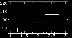
See? Easy.

More commands

erase

Clear the plot window

device postscript
device x11
list device

This command allows you to direct the output of SM to various different formats. The default is x11 which just means the screen, this is what will come up when you start SM. Type list device to get a full list of all the available options. You can use this command to get output of your plot, for example (extending the previous simple plot)

	: device postscript
	: box
	: histogram x y
	: device x11

The above commands will first redirect the output to the device postscript, then draw the graph on that device, then go back to the default device. The plot will automatically be printed out on the laser printer in room 328. Of course you don't really want to have to repeat all your commands when you need output and so we come to the next set of commands.

history

This command displays a list of the 80 most recent commands, in reverse chronological order. You can re-use a command by typing ^n where n is its number in the list

macro macro1 49 63
macro edit macro1

The first command defines a new macro called macro1 which consists of commands 49 through 63 from the history list. This sequence of commands can now be invoked very simply by typing

	: macro1

If the set of commands which make up macro1 draw a graph which you want to get a copy of you can then simply type

	: device postscript
	: macro1
	: device x11

and the plot will be printed out on the laser printer. The second command allows you to edit the macro line by line. When in macro edit mode the following keys are used:

• CTRL-X Stop editing and save the changes
• Up and down arrow keys scroll through the lines of the macro
• Left and right arrow keys scroll through each ling
• ENTER inserts a blank line after the current line
• ESC CTRL-D (press ESC once, then CTRL-D) deletes the current line

window 1 3 1 1

This command allows you to divide the plot area up into a number of sub-plots. The first two numbers in the argument are the number of divisions in the x and y direction respectively; in this case there will be 3 subplots stacked vertically. The second two arguments allow you to select one of the subplots; 1 1 corresponds to the bottommost one. You can then do all plot commands which will then appear in that subplot region, and have any number of plots on the same page.

xlabel Time (s)

Put an x-axis label on the current plot

ylabel Counts/second

Put a y-axis label on the current plot

relocate 24 43

Move to the postion (24,43) in data coordinates in the current plot

label Test

Display a label at the current position set using relocate

error_y x y err

Produce vertical errorbars at the positions defined by the points in vectors x and y of length equal to twice each value of the vector err. (The command draws an errorbar err long in both directions).

error_x x y err2

As above, but draws horizontal errorbars.

URL: http://www.phys.utas.edu.au/physics/optastr/smhelp.htm
23rd February 1998